
Equipment
Acoustic Pressure Data Acquisition and Analysis
Data Acquisition
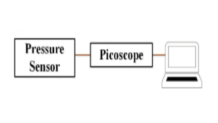
The desired pressure sensor (cavitometer, needle hydrophone, fibre-optic hydrophone etc.) is connected to a data acquisition/digital oscilloscope system such as PicoScope which is directly connected to the PC, as shown here.
Data Analysis
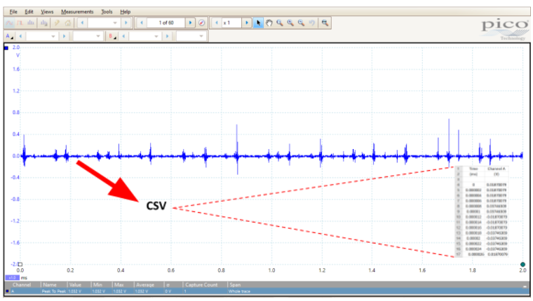
The signals in PicoScope software are saved as shown below. The signals can then be simply converted to csv file using the software (see inset). The csv files of Time vs Voltage will work as the required input files for analysis.
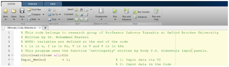
Step 1 : Click Run or press F5.
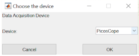
Step 2 : Choose your acquisition device: (PicoScope)
Step 3 : Input the required information in the following panel
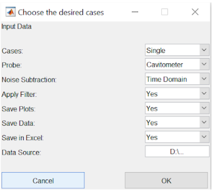
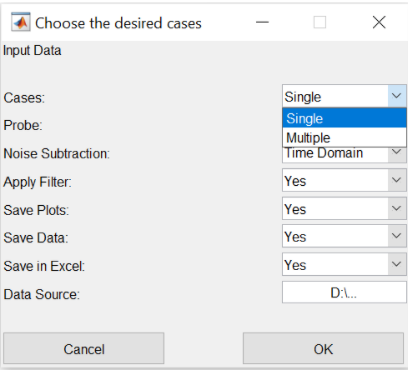
Step 4 : you can automatically analyse a single test data or multiple tests data.
Step 5 : Choose your probe for the program to use its corresponding calibration function.
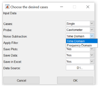
Step 6 : Choose whether you want to subtract the noise in time or frequency domain. If you do not want to subtract the noise, choose the time domain and later on in the next panel, enter 0 for noise level.
Step 7 : Choose whether you want to apply any filter to your data to discard the data outside the calibration range.
Step 8 : Choose whether you want to save your results as jpeg. For saving the results as jpeg, this program uses the advanced function export_fig. This can be downloaded from
All the function files must be placed in the main code directory or in another folder whose path should be added to MATLAB directory. If you do not have the export_fig function and choose yes, you will receive an error.
Step 9 : Choose whether you want to save the results as MATLAB dat file.
Step 10 : Choose whether you want to save the results as Excel file.
Step 11 : Paste the directory of the folder containing the csv files of the data in the last box.
Press OK.
Then another window pops up with a file name based on the sensor that you have previously chosen i.e. FIBRE-OPTIC HYDROPHONE. The next panel (for example for the case of a fibre-optic hydrophone) requires
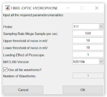
Step 12 : Select the sensor number for its calibration.
Step 13 : Sampling Rate: Enter the sampling rate of the data acquisition in Mega samples/second
Step 14 : Upper Noise Threshold: Enter the upper threshold of the noise level in mV.
Step 15 : Lower Noise Threshold: Enter the lower threshold of the noise level in mV.
Step 16 : Loading Effect: If the data acquisition device has a different loading effect than 1, enter the value here.
Step 17 : MATLAB Version: Choose your MATLAB version.
Step 18 : Number of Waveforms: If you want to analyse less number of data (csv) files than the acquired original number, untick the box and enter the desired number. If not, all data files will be used for analysis.
Press OK.
The analysis will be performed. When the calculation is over, the final results including the calibration function, original signal, maximum and RMS pressures and pressure in time domain will be both displayed on the screen and will be saved (if the user has chosen to save them).
The ultimate results as jpeg, Excel and dat file will be placed in the main directory containing the code.
Important Note: If you want to use a new sensor with its own calibration function, you should go to line 857 (Sensitivity Interpolation), follow the existing cases and open a new case, name your sensor and enter the calibration values. Then, the minimum and maximum values of frequency has to be entered in line 468 (calibration range). The new sensor name will then had to be added to the input section (for instance, for fibre-optic hydrophone, line 415).